This is the first blog-post of a series where I try to explain the inner workings of QuaggaJS an advanced barcode-reader written in JavaScript. Check out the project on GitHub and take a look at the demos, if you haven't done that already.
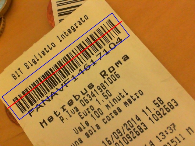
In this post, I'm going to explain how QuaggaJS locates a barcode in a given image. Let's start by examining the result of such a localization and decoding process. In the picture below you can see a blue rectangle, highlighting the position of the barcode and a red line, illustrating a successful scan. This post is all about the blue rectangle and how it is determined.
Introduction
The main purpose of a barcode locator is finding a pattern within an image which looks like a barcode. A barcode is typically characterized by its black bars and white spaces in-between. The overall size of the barcode depends on the amount of information encoded (Code128); However, a barcode can also be fixed in width (EAN13).
When we are searching for a barcode in an image we are looking for:
- lines, which are
- close to each other and
- have a similar angle.
Since locating and detecting barcodes is nothing new, the implementation is loosely based on the paper Locating and decoding EAN-13 barcodes from images captured by digital cameras. In this paper, the authors describe step by step how they solved the localization problem. Starting from there, I adapted their solution and came up with the following process:
- Create a binary representation of the image
- Slice the image into a grid (20 x 15 cells)
- Extract the skeleton of each cell
- Separate the skeleton into its parts
- Component labeling
- Calculate the rotation of each part
- Determine cell quality (rotation uniformity)
- Find connecting cells with similar rotation
- Create bounding box of connected cells
Let's get started by creating a binary image of the source.
Creating a binary image
There are many different ways of creating a binary representation of an image. The easiest way is to set a global threshold of 127 and determining for each pixel if its brighter (>=127) or darker (<127) than the threshold. While this method might be the simplest to implement, the result is usually not satisfying because it does not take into account illumination changes across the image.
In order to account for the brightness changes in the image, I chose a method called Otsu which operates on the histogram of the source image and tries to separate the foreground from the background. The image below is produced by this method.
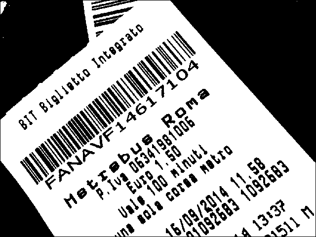
The separation of the barcode from the background works fairly well. This image will now serve as a basis for the subsequent steps.
Slicing the image into a grid
The binary image as a whole does not provide much information about its content. In order to make sense of the structure contained in the image, the latter has to be divided into smaller parts which are then described independently from each other. The resulting description is then compared with our hypothesis (lines close to each other with similar orientation) and either taken into consideration for further processing, or discarded.
A grid slicing the binary image into 20 x 15 cells seemed to work well, when assuming a 4:3 aspect ratio of the image.
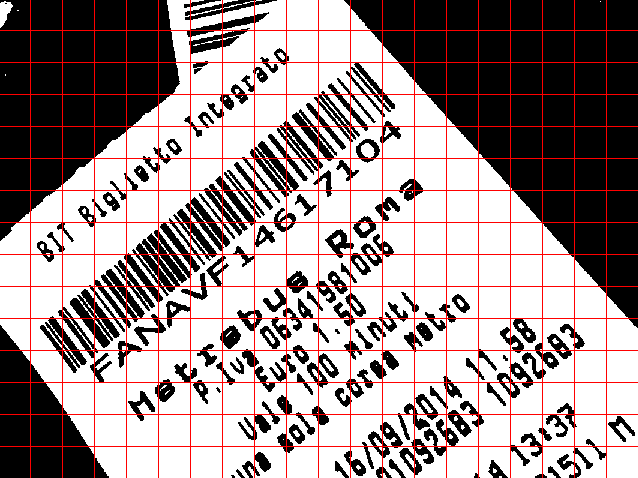
Now, each cell of the grid needs to be evaluated and classified based on the properties of our hypothesis. What this basically means is that each cell is examined to determine whether it contains nothing but parallel lines. If it does, it is considered as valuable and will be passed along to the next step. But how can we determine whether a cell contains lines which are, at best, parallel?
First of all, the bars have to be normalized in width (1px width), then separated line by line, followed by the estimation of the orientation of each line. Then, each line in the cell is compared to the others to determine the parallelity. Finally, if the majority of lines are parallel to each other, the average angle is computed. This seems like a whole lot of work, so let me explain one step after the other.
Extracting the skeleton of each cell
We start off with the normalization of the width to 1px which is done with the help of a method known as skeletonizing. This method tries to remove as much weight of each bar as possible. I managed to achieve this task by coninuously eroding and dilating the contents as long as there are unprocessed pixels. This results in a skeleton of the image as shown below:
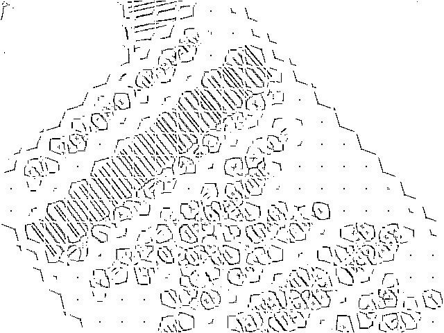
The image clearly shows the location of the barcode, and the bars of the code reduced to their minimum width of 1px. Due to the characteristics of the algorithm, some artefacts are introduced on the borders of the barcode. However, this should not bother us too much, since we allow a certain error to be present in the data being processed.
Component Labeling
In order to find out whether each cell contains parallel lines, the skeletonized content, which ideally contains straight lines of the interested area, has to be separated into individual pieces (lines). This can be achieved by applying a technique called connected-component labeling which separates a given region into its individual components. In the case of the barcode pattern, all lines within a cell are split up into single lines and then weighted by their rotation.
Due to the fact that component labeling is usually quite expensive in terms of computation, a fast algorithm was of the essence to create a real-time application. After some research, I found an implementation of the paper "A Linear-Time Component-Labeling Algorithm Using Contour Tracing Technique" by Fu Chang, Chun-Jen Chen, and Chi-Jen Lu on CodeProject. Unfortunately, the original code was written in C, so I ported it to JavaScript which took me a few hours to complete.
When applying the component-labeling algorithm to our skeletonized image, the result looks like the following.
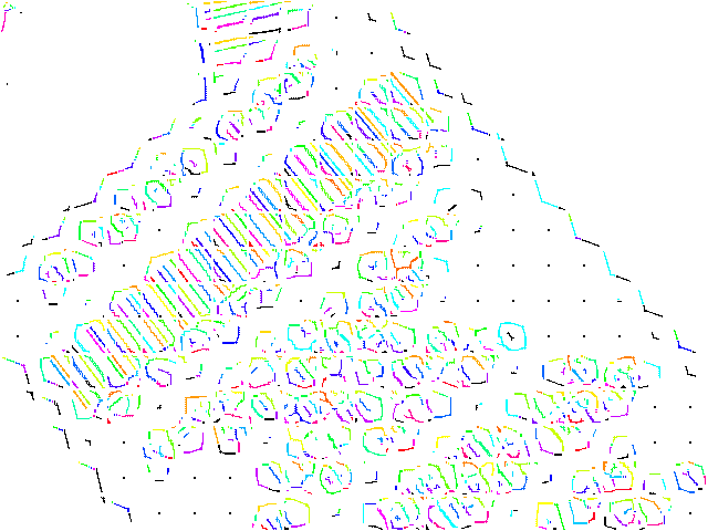
As mentioned before, each cell is treated individually, that's why each color is used repeatedly throughout the cells. The color for each component within the cell is unique and denotes the label given by the algorithm. The following images show scaled up versions of two extracted cells. The left one indicates a possible barcode area, whereas the right one does not contain much but noise.
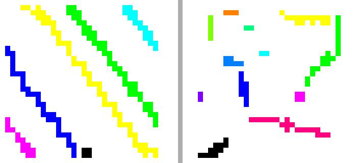
Each label can then be considered as a possible bar of a barcode pattern. To be able to classify such a representation, a quantitative value needs to be computed for each bar which can then be compared with the other components.
Determining the orientation of the components
The orientation of a single component within a cell is calculated by central image moments. This method is typically used for extracting information concerning the orientation of a binary image. In this case, the binary image is represented by the labeled components. Each component can be seen as its own binary image of which the central image moments can be computed.
As depicted in the equation below, the orientation (indicated as θ) of a binary image can be determined by its central moments (μ).

The central moments (μ) are computed using the raw moments (M) and the centroid (x,y) which (in turn) need to be calculated up front.

The following equation computes the components of the centroid (x,y) using the raw moments (M).

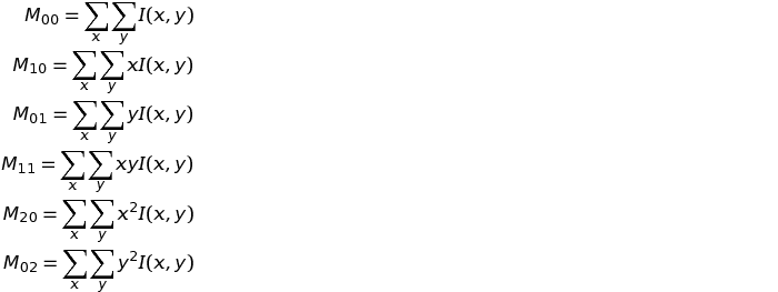
Since we need image moments up to the second order, the following listing shows the computation of each single moment. The sum over x and y denotes an iteration over the entire image, whereas I(x,y) indicates the value of the pixel at the position x,y. In this case, the value can either be 0 or 1, since we are operating on a binary image.
After this step, each component is given a property with the value of the determined angle.
Determining cell quality
Now that each cell contains components with their respective orientation, we can start classifying the cells based on those properties.
First of all, cells containing no, or just one component are discarded immediatelly and are not used for further processing. In addition, components which do not cover at least 6 px (M00) are excluded from any subsequent calculations concerning the affected cell. This pre-filtered list serves as a basis for determining the uniformity of the component's angles throughout a single cell.
In the case of a barcode, each component in a cell should be parallel to each other. However, due to noise, distortion and other influences, this may not always be the case. A simple clustering technique is applied to find out the similarity of the components containing a barcode pattern. First of all, all angles are clustered by a certain threshold, whereupon the cluster with the highest count of members is selected. Only if this cluster's member-size is greater than 3/4-th of the initial set this cell is finally considered as being part of a barcode pattern. From now on, this cell is referred to as a patch, which contains the following information:
- an index (unique identifier within the grid)
- the bounding box defining the cell
- all components and their associated moments
- an average angle (computed from the cluster)
- a vector pointing in the direction of orientation
The following picture highlights the patches (cells) which were classified as a barcode pattern.
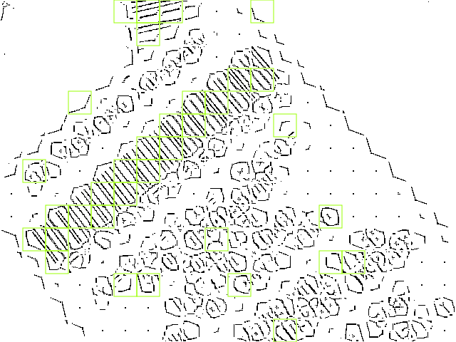
As can be seen in the image above, some cells were falsely classified as being part of a barcode pattern. Those false positives can be detected by simply finding adjoining areas (consisting of more than one cell) and discarding all the remaining ones.
Finding connected cells
Basically, cells can be considered as being part of a barcode, if they are neighbors and share common properties. This grouping is done by a simple recursive component-labeling algorithm which operates using similarity of orientation. In order for a patch (component) to be considered as amember of a label, its vector must point in the same direction as its neighbor's vector. To account for deviations caused by distortion and other geometric influences, the orientation can deviate up to 5 %. The image shown below illustrates connected cells where the color defines the link to a certain group.
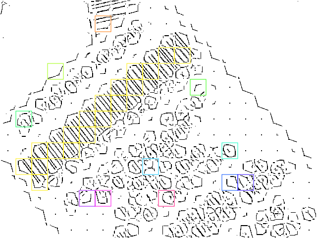
The only group containing more than one patch is the yellow one. Sometimes even neighboring cells are colored differently. This happens if the orientation of those patches differ too much (> 5%).
Selecting groups
Next we try to identify those groups which are most likely to contain a barcode. Since more than one barcode can be present in an image at the same time, the groups are first sorted and then filtered by their number of members (patches).
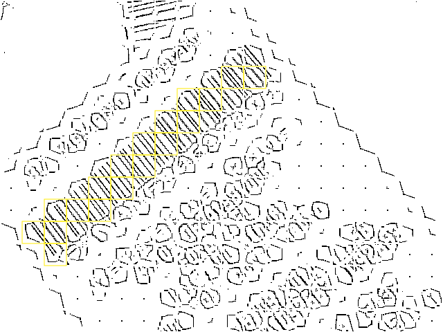
In the example shown above, only the yellow group remains and is passed on to the next step, the creation of a bounding-box.
Creating a bounding box
Finally, all the information necessary for outlining the location of the barcode is available. In this last step, a minimum bounding box is created which spans over all the patches in one group. First of all, the average angle of the containing patches is calculated which is then used for rotating the cells by this exact angle. After that, a bounding box is computed by using the outermost corners of all the patches.
Finally, the bounding box is rotated in the inverse direction to transform it back to its origin. The result is shown in the image below.
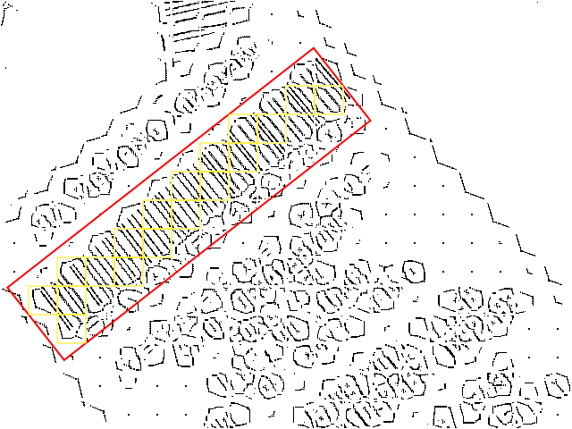
As illustrated in the image above, the bounding box is placed exactly where the barcode pattern is printed.
Further Work
Now that we know how to locate a barcode-like pattern in an image, it's time to move on to the next step, the process of decoding the code. Since we already know where the barcode is located, this task is rather easy compared to what you just read. All this and more is going to be part of the next post of this series.
Thanks for reading my post I hope you enjoyed it as much as I enjoyed working on QuaggaJS.